Will I have some theme for these posts?
The question is, again, rather easy to state. But to me, it is one of the best introductory examples to ODE solving and chaos with a simple physical model.
Q1. Describe the motion of a simple pendulum were you to replace the massless string with a spring of force constant k.

Note that the Lagrangian formulation (which I’d never correctly spell without autocorrect) allows us to escape the consideration of various inertial forces, and is hence preferred.
Suppose we start from rest and horizontally, we may use numerical ODE solver to grasp the full behaviour.
But wait, before that, can we ‘eyeball’ some features of this system?
Yes we can!
Due to the important role that the ratio k/m plays, we call it Omega(x)^2, which stands for the natural oscillation frequency of spring, squared.
When this value tends to infinity, the spring is effectively rigid, and the problem degenerates into the regular pendulum model.
When this value tends to zero, however, the motion will simply tend to that of a free fall.
The two natural frequencies intrinsic to the system, Omega(theta) and Omega(x), will resonate with some settings, leading to interesting resonant behaviours.
OK, it’s time for Python to take over… Feel free to try and modify the script below for yourselves. Note that you need a Python3 environment with numpy, matplotlib and scipy installed.
# -*- coding: utf-8 -*-
"""
Created on Wed Dec  5 18:05:27 2018
OVEAL est. 2017
@author: FVW, for distribution on ftdsci.com.
"""

# Let's start #

import numpy as np
from scipy.integrate import odeint
from matplotlib import pyplot as plt
from matplotlib import animation

plt.rcParams["figure.figsize"] = [10,10]

# Global Variables #

g = 10
timestep = 0.01
l = 1.5

OmegaThSq = 3

def OmegaXSq(x):
    global g, l
    return g/(l+x)

# ODE System #
def SpringPendulum(x,t):

    xdot = x[1]
    xddot = (l+x[0])*x[3]**2+g*np.cos(x[2])-OmegaThSq*x[0]
    thdot = x[3]
    thddot = -2/(l+x[0])*x[1]*x[3]-OmegaXSq(x[0])*np.sin(x[2])
    return np.array([xdot,xddot,thdot,thddot])


tout=np.arange(0,9725,timestep)

cool=odeint(SpringPendulum,[0,0,np.pi/2,0],tout)

Radius = l+cool[:,0]
Theta = cool[:,2]

Plotx = Radius*np.sin(Theta)
Ploty = -Radius*np.cos(Theta)

plt.plot(Plotx,Ploty)


# Now, Animating in the 2D plane #

fig = plt.figure()
ax = fig.add_subplot(111, aspect = 'equal', autoscale_on=False, xlim=(-6, 6), ylim=(-12, 0))
ax.grid()

lineorig, = ax.plot([], [], 'o-', lw=2)
line, = ax.plot([], [], 'ro', lw=2)
bigmass, = ax.plot([], [], 'go', lw=2)
time_template = 'time = %.1fs'
time_text = ax.text(0.05, 0.9, '', transform=ax.transAxes)

def init():
    lineorig.set_data([], [])
    line.set_data([], [])
    time_text.set_text('')
    return line, lineorig, time_text

def animate(i):
    x = [0,Plotx[i]]
    y = [0,Ploty[i]]
    a = [Plotx[i]]
    b = [Ploty[i]]
    lineorig.set_data(x, y)
    line.set_data(a,b)
    bigmass.set_data(0, 0)
    return lineorig, line, bigmass

ani = animation.FuncAnimation(fig, animate, np.arange(1, 999),
                              interval=25, blit=True, init_func=init)

ani.save('PendulumSpringDemo.mp4', fps=30)
plt.show()
Sample solution gallery
For the plots below, we (non-dimensionalised) and assigned the following constant values:
l = 2
g = 10
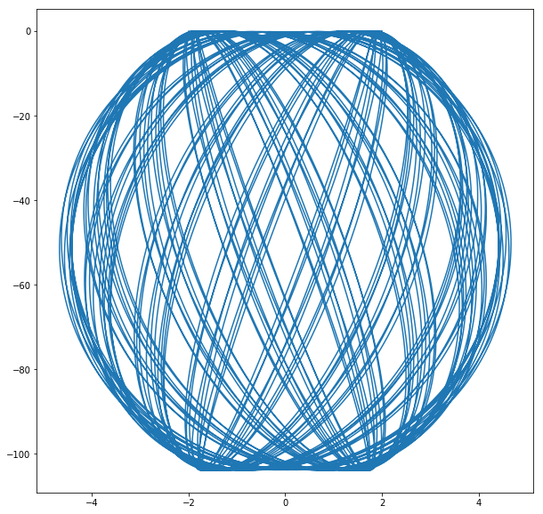
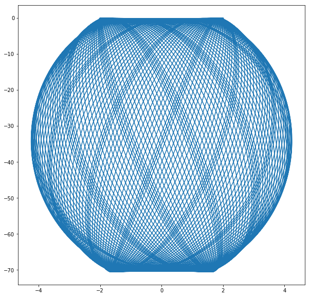
omega^2 = 0.3
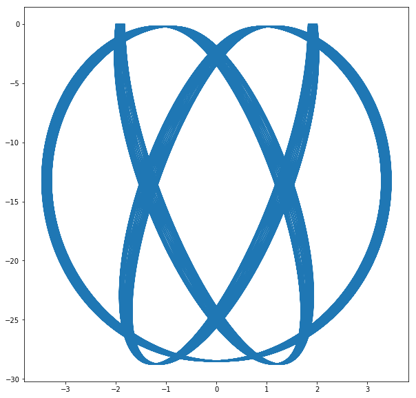
omega^2 = 0.8
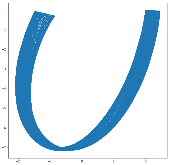
omega^2 = 5

omega^2 = 10000
Problem solved, somewhat.
A few bits of website design notes, I guess.
First of all, I desperately need a website setting that supports LaTeX… maybe… Donate to me so I can afford to seek my own hosting service?
Then, there’s color choice considerations… I will produce the future plots and writings in dark color palettes.
